2.3.2 Critical Angle

Figure 24.  Critical Angle (1)

If we consider Figure 22 on page 40 we notice that as the angle θ₁ becomes larger and larger so does the angle θ₂. Because of the refraction effect θ₂ becomes larger more quickly than θ₁. At some point θ₂ will reach 90º while θ₁ is still well less than that. This is called the “critical angle”. When θ₁ is increased further then refraction ceases and the light starts to be reflected rather than refracted.

Thus light is perfectly reflected at an interface between two materials of different refractive index iff:

1.  The light is incident on the interface from the side of higher refractive index.

2.  The angle θ is greater than a specific value called the “critical angle”.

If we know the refractive indices of both materials then the critical angle can be derived quite easily from Snell’s law. At the critical angle we know that θ₂ equals 90º and sin 90º = 1 and so:

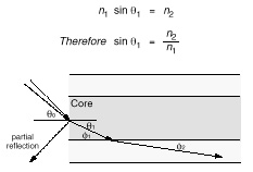
Figure 25.  Critical Angle (2)

If we now consider Figure 24 and Figure 25 we can see the effect of the critical angle within the fibre. In Figure 24 we see that for rays where θ₁ is less than a critical value then the ray will propagate along the fibre and will be “bound” within the fibre. In Figure 25 we see that where the angle θ₁ is greater than the critical value the ray is refracted into the cladding and will ultimately be lost outside the fibre.

Another aspect here is that when light meets an abrupt change in refractive index (such as at the end of a fibre) not all of the light is refracted. Usually about 4% of the light is reflected back along the path from which it came. This is further discussed in 2.1.3.2, “Transmission through a Sheet of Glass” on page 22.

When we consider rays entering the fibre from the outside (into the endface of the fibre) we see that there is a further complication. The refractive index difference between the fibre core and the air will cause any arriving ray to be refracted. This means that there is a maximum angle for a ray arriving at the fibre endface at which the ray will propagate. Rays arriving at an angle less than this angle will propagate but rays arriving at a greater angle will not. This angle is not a “critical angle” as that term is reserved for the case where light arrives from a material of higher RI to one of lower RI. (In this case, the critical angle is the angle within the fibre.) Thus there is a “cone of acceptance” at the endface of a fibre. Rays arriving within the cone will propagate and ones arriving outside of it will not.

In Figure 25 on page 41 there is a partial reflection present when most of the light is refracted. This partial reflection effect was noted earlier in 2.1.3.2, “Transmission through a Sheet of Glass” on page 22. These reflections are called “Fresnel Reflections” and occur in most situations where there is an abrupt change in the refractive index at a material interface. These reflections are an important (potential) source of disruption and noise in an optical transmission system. See 2.4.4, “Reflections and Return Loss Variation” on page 67.

2.3.3 Numerical Aperture (NA)

Figure 26.  Calculating the Numerical Aperture

One of the most often quoted characteristics of an optical fibre is its “Numerical Aperture”. The NA is intended as a measure of the light capturing ability of the fibre. However, it is used for many other purposes. For example it may be used as a measure of the amount of loss that we might expect on a bend of a particular radius etc.

Figure 24 on page 41 shows a ray entering the fibre at an angle close to its axis. This ray will be refracted and will later encounter the core-cladding interface at an angle such that it will be reflected. This is because the angle θ₂ will be greater than the critical angle. The angle is greater because we are measuring angles from a normal to the core-cladding boundary not a tangent to it.

Figure 25 on page 41 shows a ray entering at a wider angle to the fibre axis. This one will reach the core-cladding interface at an angle smaller than the critical angle and it will pass into the cladding. This ray will eventually be lost.

It is clear that there is a “cone” of acceptance (illustrated in Figure 26). If a ray enters the fibre at an angle within the cone then it will be captured and propagate as a bound mode. If a ray enters the fibre at an angle outside the cone then it will leave the core and eventually leave the fibre itself.

The Numerical Aperture is the sine of the largest angle contained within the cone of acceptance.

Looking at Figure 26 on page 42, the NA is sin θ₀. The problem is to find an expression for NA.

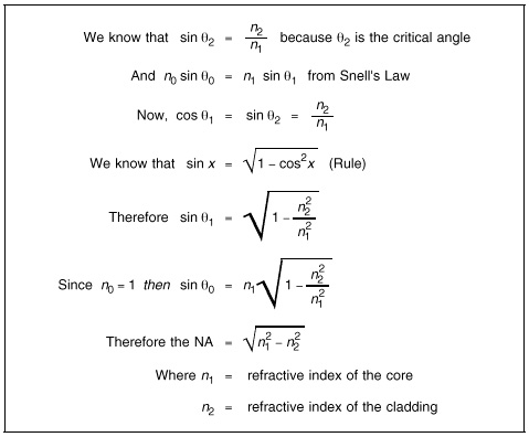
Another useful expression for NA is: NA = n₁ sin θ1. This relates the NA to the RI of the core and the maximum angle at which a bound ray may propagate (angle measured from the fibre axis rather than its normal).

Typical NA for single-mode fibre is 0.1. For multimode, NA is between 0.2 and 0.3 (usually closer to 0.2).

NA is related to a number of important fibre characteristics.

1.  It is a measure of the ability of the fibre to gather light at the input end (as discussed above).

2.  Because it is a measure of the contrast in RI between the core and the cladding it is a good measure of the light guiding properties of the fibre. The higher the NA the tighter (smaller radius) we can have bends in the fibre before loss of light becomes a problem.

3.  The higher the NA the more modes we have! Rays can bounce at greater angles and therefore there are more of them. This means that the higher the NA the greater will be the dispersion of this fibre (in the case of MM fibre)!

4.  In SM fibre a high RI contrast usually implies a high level of dopant in the cladding. Since a significant proportion of optical power in SM travels in the cladding we get a significantly increased amount of attenuation due to the higher level of dopant. Thus (as a rule of thumb) the higher the NA of SM fibre the higher will be the attenuation of the fibre

2.3.4 Propagation Modes

So far our description of light propagation in a multimode fibre has used the classic “ray model” of light propagation. While this has provided valuable insights it offers no help in understanding the phenomenon of “modes”.

Figure 27.  Multimode Propagation. At corresponding points in its path, each mode must be in phase with itself. That is, the signal at Point A must be in phase with the signal at Point B.

When light travels on a multimode fibre it is limited to a relatively small number of possible paths (called modes). This is counter to intuition. Reasoning from the ray model would lead us to conclude that there is an infinity of possible paths. A full understanding of modes requires the use of Maxwell’s equations which are very difficult and well outside the scope of this book.

A simple explanation is that when light propagates along a particular path within a fibre the wavefront must stay in phase with itself. In Figure 27 this means that the wave (or ray) must be in phase at corresponding points in the cycle. The wave at point A must be in phase with the wave at point B. This means that there must be an integer multiple of wavelengths between points of reflection between the core and the cladding. That is, the length of section 2 of the wave in the figure must be an integer number of wavelengths long. It is obvious that if we have this restriction on the paths that can be taken then there will be a finite number of possible paths.

Figure 15 on page 33 shows the usual simplistic diagram of modal propagation in the three common types of fibre. We must realise however that this is a two dimensional picture and we are attempting to represent a three-dimensional phenomenon! Many modes are oblique and spiral in their paths. In fact the majority of modes never intersect with the fibre axis at any time in their travel! This is illustrated in Figure 28 on page 45.

Figure 28.  Spiral Mode. In MM GI fibre most modes have spiral paths and never pass through the axis of the fibre. In much of the literature these modes are also called “corkscrew”, “screw” or “ helical” modes.

Perhaps the most important property of modes is that all of the propagating modes within a fibre are orthogonal. That is, provided that the fibre is perfect (perfectly regular, no faults, perfectly circular, uniform refractive index...) there can be no power transfer or interference between one mode and another. Indeed this is the basic reason for the restriction (stated above) that corresponding points along the path of a mode must be in phase. If they were not then there could be destructive interference between modes and the wave could not propagate.